In Praise of Slowness
How using a slow computer can help us to refine our programming skills.
It's often considered wise to impose restrictions on the devices that learners can use - new motorcyclists, for example, are limited to machines of up to 50cc. My first car was a 998cc Metro (in the days before turbochargers were common, this developed 42bhp) - it taught me to carefully assess gaps in traffic, and how to judge corners to reduce braking (and therefore loss in momentum).
Early in my degree course, we were told that the advent of cheap and powerful devices will set software engineering back 25 years. It's a quotation that that they attributed to Dijkstra, but I haven't managed to verify the source.
I initially learnt to program on a computer with a 3.5MHz processor and 1kB of RAM. In those days we were very careful about efficiency, commonly kept use of variables to a minimum, etc. You might have read articles about how developers struggled to fit large games, such as The Hobbit, into the RAM available in 80s home computers. Because of this, even now, I often have an idea for a program or web-page, such as the Image Manipulator, think that it'll never work due to the amount of data generated... only to find that it works happily on my phone.
Efficiency
Needing to think about efficiency, however, is a big benefit of using a slower device and the reason that you should consider trying one. Efficiency is something that's often overlooked in current programming courses, but it's very important to computer scientists. I mentioned in a previous blog that after a discussion about efficiency in a teachers' forum, an optimised version of a program took pretty-much the same amount of time to run on my Windows PC as the original version that looped thousands more times - both took a few hundred milliseconds. Running the two programs on a BBC Model B emulator, however, really showed the difference - one took 0.13s and the other took over a minute.
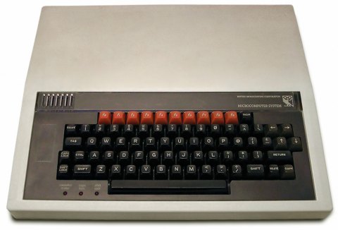
When Computing was added to the National Curriculum, my first thought was that BBC BASIC was the way to go - there are compiled emulators that you can download and web-based ones that will work on Chromebooks. The only thing that put me off was the difficulty of editing and saving the programs. I still use the BBC Model B for some demonstrations, though.
Try It Yourself
You can download and install BeebEm for Windows or use an on-line emulator such as jsbeeb. Both are compatible with floppy disc images that you can find on-line, include things like Elite if you're a retro-gamer. You can download my circles programs and use them for demonstrations and investigations. You can also read more about the maths behind drawing circles if you're not familiar with the techniques.
With either emulator, the first step is to load the disc image. In BeebEm this is done using the File menu to Load Disc 0. In jsbeeb it's done using the Discs menu and choosing From examples or local.
DFS Basics
The BBC Model B runs an operating system called DFS (Disc Filing System) that has a command-line interface. These are the key commands that you can use for your demonstration/investigation:
- *CAT shows the contents of the current disc (like dir in DOS/Windows or ls in Unix/Linux). [NB. The * is not a typo!]
- LOAD loads a program from the disc. The filename is enclosed in speech marks, e.g. LOAD "TRIG".
- SAVE saves a program to the disc (e.g. if you want to keep any changes). The filename is enclosed in speech marks, e.g. SAVE "NEWTRIG".
- LIST shows the code of the current program.
- RUN runs the current program.
- RENUMBER renumbers the lines of code to multiples of ten, should you need to insert any new lines (which can be sequenced by giving them an appropriate number).
If you are familiar with other types of BASIC, such as GW Basic, Visual Basic, Small Basic, etc., then BBC BASIC should look familiar. With a knowledge of Python and ERL you should be able to work out what the programs are doing even if you aren't familiar with BASIC.
Comparisons
You can compare the programs for drawing the circles using two main criteria and show your students the impact of changing both the number of calculations and the complexity of those calculations.
Number of Repetitions
All programs make use of loops:
- the programs with TRIG in the name loop from 0 to 360 (i.e. for each degree in the circle)
- the programs with PYTHAG in the name loop twice from -400 to 400 (this represesents the x-coordinate), i.e. 1600 repetitions altogether
- the RANDOM programs let you choose the number of repetitions directly
The PYTHAG and PYTHAG programs ask you for a Step size, which is used in the loop. You can therefore compare the timings for the same number of repetitions, e.g. if you use a step size of 9 with TRIG, a step size of 40 with PYTHAG and 40 repetitions in RANDOM.
Complexity of Calculations
Each program uses a different type of calculation:
- TRIG uses trigonometry - i.e. sines and cosines - to calculate the co-ordinates
- PYTHAG uses Pythagoras - i.e. square roots - to calculate the co-ordinates
- RANDOM uses only arithmetic to calculate the co-ordinates
You should see that the sine and cosine calculations take longer. The files with the number suffixes contain programs that reduce the number of complex calculations by taking advantage of symmetry - TRIG2, PYTHAG2 and RANDOM2 both use the complex calculations to calculate the coordinates for only half the circle and then simple arithmetic to reflect the coordinates for the other half. TRIG3 and PYTHAG3 both take this a step further by calculating the co-ordinates for a quarter of the circle and then reflecting them in both directions.
Circle Conclusion
By tweaking the number of calculations and the type of calculation used, you should be able to reduce the time taken for drawing the circle from 20-odd seconds to less than 1s - an improvement you'd be unlikely to see on a modern PC. And you'll give your students a taste of computing history!
Demonstrating Big O
Slow computers are also good for demonstrating Big O - the time complexity of an algorithm. This is not the amount of time that a program takes to run - that would depend on the performance of the device. The best way to think of Big O is how much longer the program will take if you run it on a larger dataset.
Big O is usually expressed as a function of n, where n is the multiplier for the number of times you've increased the size of the dataset - e.g. if you are processing twice as many items, n will be 2. A bubble sort, for example, has a time-complexity of O(n²), so if we're sorting twice as many items it will take four (2²) times as long. If we're sorting ten times as many items, it will take 100 (10²) times as long, if we're sorting 1000 times as many items it will take one million (1000²) times as long, and so on.
Using a fast computer, these increases might not be noticeable - if sorting ten items takes a few milliseconds, then sorting 20 items will also take milliseconds. If, however, sorting a small number of items takes a few seconds then we start to see quite a delay when we increase the amount of data.
You can still see a big difference on a modern computer if you greatly increase the amount of data, of course. The Advent of Code tasks, for example, quite often have a small amount of data that can be processed to test your program, then a much larger set of data to process for the answer. It can sometimes be the case that the examples take a negligible amount of time to process, but the full dataset takes hours.
Sorting Algorithms
The sorting disc image contains the following files:
- BUBBLE, which is a bubble sort program
- SELECT, which is a selection sort program
- INSERT, which is a insertion sort program
- QUICK, which is a quicksort program
These can be loaded using the same DFS commands as the circle programs (see above). Each will ask you how many items you want to sort and then will perform sorts on that number of items, organised as follows:
- a set of integers in reverse order - e.g. if you choose ten items, for example, the program will sort a set containing 9, 8, 7, 6, 5, 4, 3, 2, 1 and 0
- a same-sized set of random integers - e.g. if you choose ten items the program will sort ten random integers
The items to be sorted are stored in an array and each program contains a procedure called PROCPRINTARRAY that displays its contents. You can either add calls to this procedure in the program, or run it after the program has finished by typing PROCPRINTARRAY at the command prompt.
You should notice that the random integers are generally quicker to sort as there will be fewer swaps required. The time for the random set will vary depending on the numbers chosen, but you could run the program several times and take the average.
Even sorting a small number of items - e.g. ten - will take a noticeable amount of time. You can then sort a larger set - e.g. twice as many - and see how long that takes. It's also interesting to note that although bubble and selection sorts are both O(n²), they don't take the same amount of time. That's because coefficients are omitted, so n² and 100n² are both written as n².
Watch a video of me doing this demonstration on YouTube.
This blog was originally written in October 2023 and was updated in November 2023 to add the Quicksort program.